


|
|
|
G.Bergeles (a), I.Glekas (b), J.Prospathopoulos (a), S.Voutsinas (a)
(a) National Technical University of Athens
Department of Mechanical Engineering, Fluids Section
P.O.box 64070, Zografou, Athens, Hellas
Fax: +301-772-1057, Tel :+301-772-1096, e-mail: aiolos@fluid.mech.ntua.gr
(B) Environmental Management Consultants
P.O. Box 1559-1510, Nicosia, Cyprus
Fax: +357-2-456607, Tel: +357-2-456665
KEYWORDS: Siting, Navier-Stokes equations, terrain, grid.
2. REQUIREMENTS OF A DESIGN TOOL AND MODEL CAPABILITIES
Siting refers to the procedure of determining the most windy spots in a relatively large region, where wind turbines can be erected. At those spots not only the mean wind speed but also the expected energy production (wind potential) should be high. The wind potential can be estimated either by means of direct measurements or by means of modelling. When modelling is used the calculation is steady in the sense that the flowfield is calculated assuming constant external conditions.
Because of their low computational cost simple models [1,2,3] are in almost exclusive use. However, in several cases they fail to give good predictions so more detailed models such as Navier-Stokes models [4,5] have been proposed. Navier-Stokes models require considerable computational effort which has been a serious drawback for their wide use. Even so, they constitute the most complete approximation and so they could be useful at least for checking and calibrating simpler models. The fast computer development will lead to an analogous decrease in the computational cost of Navier-Stokes models. Therefore, it is worth checking the confidence limits of Navier-Stokes models when computational cost is restricted. Such an implication can lead to the best possible compromise between computational cost and reliable predictions.
An investigation was carried out with respect to these two points out using a fully 3D turbulent Navier-Stokes solver. In the present paper we report the key findings and results of this work.
2. REMARKS ON THE NUMERICAL MODEL & ITS USAGE FOR SITING
The flow problem in hand is governed by the turbulent steady 3D Navier-Stokes equations. The set of equations is solved by means of the finite-volume method (See [6] for details). A well-known difficulty is the imposition of correct boundary conditions. In the case of siting, the ground is regarded as the bottom of the computational box. Assuming that we align the grid with the inflow we can distinguish:
The inlet plane, i.e. the side where from the fluid inflows the domain. The inflow profile is considered as a well developed boundary layer which follows a logarithmic law (or an exponential law) with given maximum velocity.
The outlet plane, i.e. the side where from the fluid outflows the domain. If there is no specific information boundary conditions of full development of the flow (Neumann conditions) are imposed.
The top plane is regarded as a plane well out of the boundary layer so constant flow conditions can be set.
The lateral planes: Dirichlet or Neumann conditions are imposed depending on the available information.
In the case of a really complex terrain neither the Dirichlet nor the Neumann conditions can be considered correct. Such boundary conditions can be considered well-fitted only if a sufficiently large part of the terrain close to the boundaries is smooth. This can be accomplished by artificially extending the computational domain. If the terrain is really complex a "nesting" procedure is applied.
A significant parameter which affects directly the computational cost of the method is the density of the computational grid. We did not expect to achieve grid independent solutions for 3D full scale flows. Instead we tried to define the best possible compromise between computational cost and reliable predictions through a parametric analysis.
Eight cases were considered in total. They correspond to different topographies of varying complexity and wind conditions from all over Europe. In order to better understand the numerical behaviour of the flow model, a simple case, the Askervein site in U.K. for which extensive measurements exist [7], was first considered (Fig 1).
Boundary conditions: In order to cancel the external perturbations the terrain is extended to a flat level. In some cases this is combined with a smoothening of the irregularities in the border region. The artificial upstream extension of the terrain permits the full development of a turbulent boundary layer. In the case of the Askervein site this improves the predictions significantly just in front of the hill (Fig 5).The artificial downstream extension of the terrain permits a more complete recovery of the flow. By extending the terrain laterally the restriction of the flow by the borders is avoided (Fig 6).
In case the site under consideration is part of a very complex terrain, a confined computational box would present steep irregularities along its borders. In this case the predicted flow field can become even unrealistic. In particular, the velocity over the spots of high altitudes located close to the borders is considerably underestimated. These strange predictions close to the boundaries affect more or less the predictions over the whole region. A way to overcome these difficulties is the use of a nested sequence of grids. Nesting was applied to four terrains of high complexity and it led to reasonable predictions. Indicative results concerning the Zartener Becker site are presented in Fig 11 (no nesting) and Fig 12 (nesting). The differences between the two cases are obvious in the regions located close to the borders. Grid density: The predictions remain grid dependent in the vertical direction even for the densest grid (Fig 2). This dependence decreases with the height. At 60m A.G.L. there is no significant difference in the predictions between the two finest grids ( not shown here, see [8]) with the exeption of the recirculation zone. Because recirculation zones are not suitable for wind energy applications we conclude that a vertical density around 80-100 points will give satisfactory overall results. The contours of the total velocity for a grid with 80 points in the vertical direction are shown in Fig 3.
The refinement of the grid in the main direction of the flow changes the topography due to the interpolation made in order to calculate the altitudes of the additional grid points. This can lead to important local differences. The refinement of the grid in the lateral direction induces no significant change to the predictions.
In an attempt to combine the artificial extension of the terrain with a sufficient but reasonable grid density as regards the computational cost, a compromise was sought. The terrain was artificially extended all along its borders and the grid was finer in the region of the real "terrain" (Fig 4: Askervein, Fig 8: Andros, Greece). The grid contained about 300000 grid-points in total. Results are presented in Fig 5,6 for the Askervein site in U.K. and in Fig 9 for the Andros site in Greece. In the case of the Askervein site (Fig 5) it is noted that the dimensionless velocity over the hill top is about equal to 1.6 (significantly lower than 2) showing a strong 3D behaviour. In the case of the Andros site which is a complex terrain the predictions can be considered to mbe in good agreement with the mesurements [1] (Fig 9).
Computational cost - Performance
A drawback to all detailed models is their high computational cost. This is due to the complexity of the Navier-Stokes equations as well as the large grid sizes used in order to get physical and accurate results. However, the use of the methodology is feasible within the framework and the limitations set by the "Best Possible Choice". It is an optimum compromise between giving consistent predictions of acceptable quality with limited computational cost. A typical run requires 48h on a Workstation running at 200 Specfp92 (The fastest processor nowadays runs at 600 Specfp92).
In terms of cost reduction, the "nesting" procedure saves a quite good part of the overall amount of computational cost. An alternative which is currently in progress is the use of parallel processing.
Summarising the work, certain guidelines concerning the use of a Navier-Stokes methodology in complex terrains can be provided. The imposition of accurate boundary conditions is of crucial importance and was examined thoroughly. When the terrain is smooth close to its borders an artificial extension is acceptable and leads to satisfactory predictions ("Best Possible Choice"). In case the terrain is really complex, the "nesting" procedure is proposed to handle the problem of imposing appropriate boundary conditions. According to this, we start the calculations from a wide region and then focus on the region of interest.
Nesting can be generalized to a sequence of more than two grids. Calculations will start with a really wide region and focus step by step towards smaller regions. Thus, the influence of the surrounding topography, which plays an important role in the shaping of the wind profile and consequently in the determination of the boundary conditions, could be taken into account.
As regards the wind potential estimation, it is deduced that the Navier-Stokes methodology via the "nesting" procedure is capable of predicting well the velocity field over complex terrains. However, it demands a great deal of computational time and data in comparison to simpler methodologies. In this connection two remarks can be made: First, there is no need for using particularly large grid sizes in order to make an estimation of the wind potential which will lead to the choice of the proper spotss for wind turbine installation. Second, a further significant reduction of computational time can be achieved using parallel processing in order to make the methodology applicable for engineering applications.
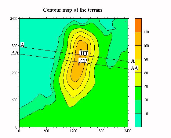
Figure 1: Askervein - Contour map of the terrain
HT: Hill top ( first reference location )
CP: Centre point ( second reference location )
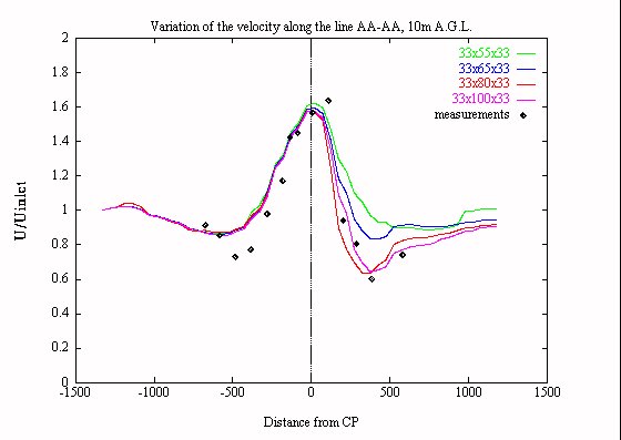
Figure 2: Askervein - Variation of the total velocity along the intersection AA-AA for various grid densities in the vertical direction
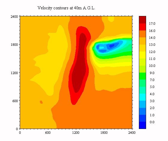
Figure 3: Askervein - Contours of the total velocity at 40m A.G.L., grid 33x80x33
Figure 4: Askervein - The "Best Possible Choice", digitized terrain 75x45
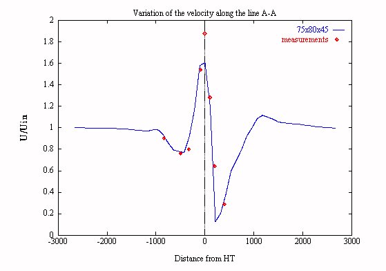
Figure 5: Askervein - The "Best Possible Choice", variation of the total velocity along the intersection A-A, grid 75x80x45 ( 10m A.G.L.)
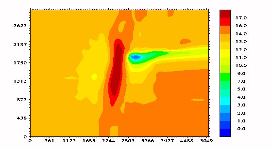
Figure 6: Askervein - The "Best Possible Choice", contours of the total velocity at 40m A.G.L., grid 75x80x45
Figure 7: Andros - Digitized modified terrain, 33x33
Figure 8: Andros - The "Best Possible Choice", digitized terrain 75x55
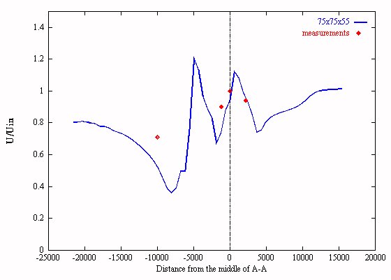
Figure 9: Andros - The "Best Possible Choice", variation of the total velocity along the intersection A-A, grid 75x75x55
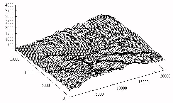
Figure 10: Zartener Becker - Contour map of the wider terrain (Hollental)
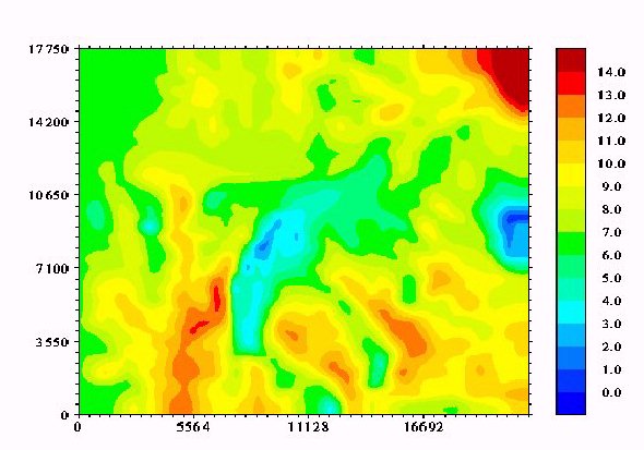
Figure 11: Zartener Becker - Contours of the total velocity at 40m A.G.L., no nesting
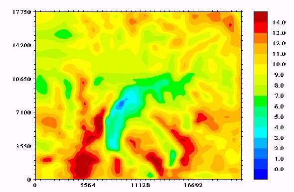
Figure 12: Zartener Becker - Contours of the total velocity at 40m A.G.L., nesting
 |
 |
 |
 |
 |