


|
|
|
D. G. Triantos, K. Pothou
National Technical University of Athens, Fluids Section,
PO Box 64070, 15710 Zografou, Athens, Greece
tel.:(+)301-7721096, fax:(+)301-7721057, e_mail: aiolos@fluid.mech.ntua.gr
In order to approximate the velocity field in C.F.D. applications using Langragian approaches, pointwize methods using particles have been introduced. These methods are sufficiently accurate inside their limitations, due to the existence of analytical expressions for the velocity field in most cases. However the computational cost of the particle method is prohibitive for applications which need large numbers of particles, for example applications of unsteady phenomena. In order to overcame this difficulty Particle Mesh methods have been introduced. These methods lead to a significant time gain for slightly less accuracy. However the study of complex unsteady phenomena demand large amounts of computational time even with the use of Particle Mesh methods.
Today 's availability of concurrent computers show a way to brake through the problem. In this work we shall try to present a concurrent Particle Mesh method suitable for distributed memory machines. In our attempt to develop a code that will run efficiently without any changes in a wide range of parallel computers as well as in a network of serial computers under a message passing platform we used the BLACS interface [1].
Particle Mesh algorithm and parallelization strategy
Suppose that we have a set of particles of total number NP, which are determined in the computational space Vp, by their position Xi={ xi,yi,zi} i=1...NP, and their intensity G={gxi,gyi,gzi} i=1..NP. In order to calculate the velocity and the deformation of each particle with a Particle Mesh method the next steps should be followed.
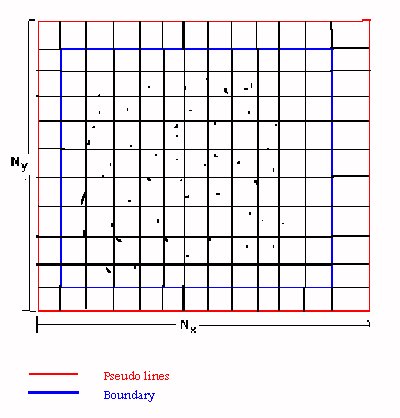
Figure 1
Figure 2
Suppose that NPR is the number of processors that can be used. The first step is to divide the mesh so that each processor takes a part of it and the corresponding particles that exist in that part. The division should be in a way that all processors take equal nodes and equal particles as possible, so all processors carry the same load. Suppose that the mesh is rectangular the division could be according the {Fig 3} in one or in two dimensions. The optimum way is related with the number of the available processors.
In the partition of the grid corresponding to processor, few grid lines (usually two) should be added at each edge at the direction of the division so that the boundary of each partition is sufficiently far from the included particles {Fig 4}. These additional grid lines are necessary for the accuracy of the results but also give an additional overhead. If the extrapolation method we used demand an extra grid line (pseudo line) out of the border this should be added too.
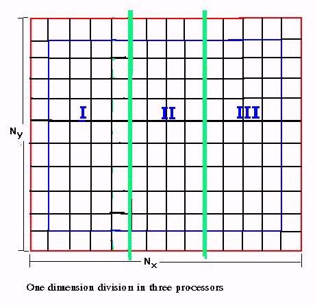
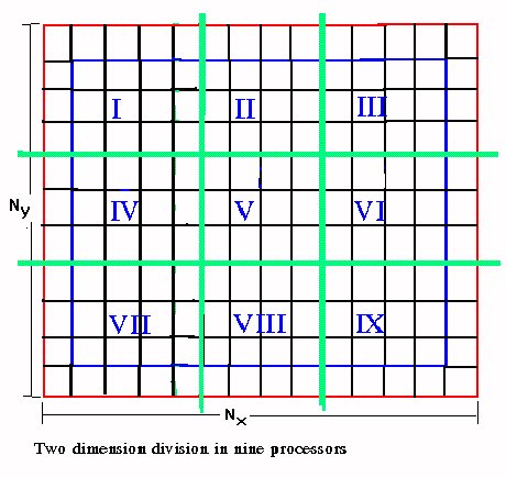
Figure 3
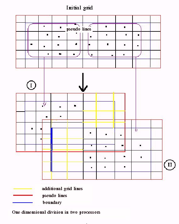
Figure 4
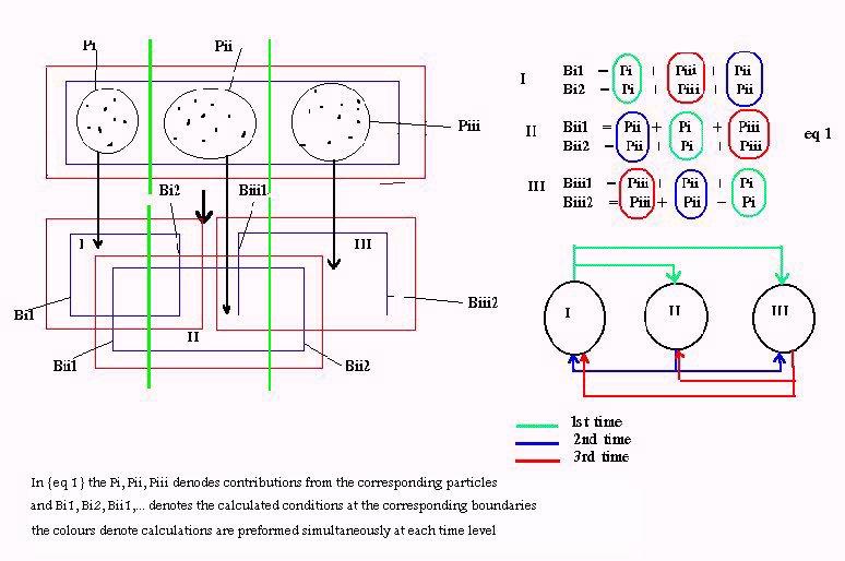
Figure 5
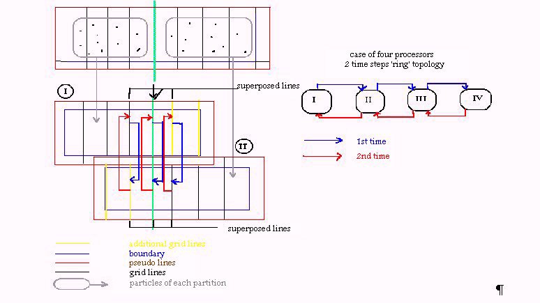
Figure 6
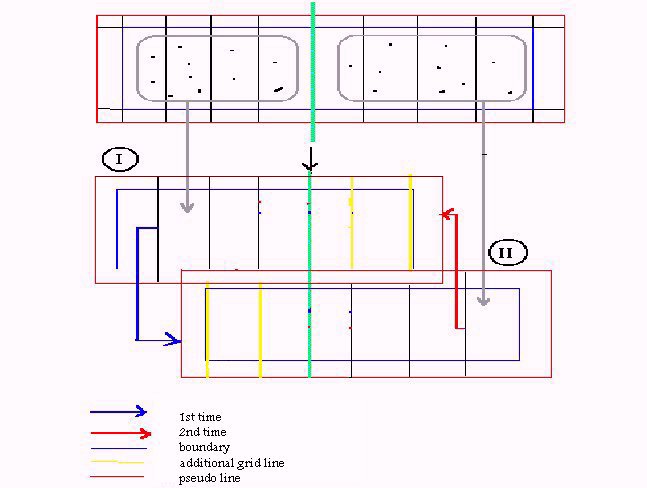
Figure 7
In order to estimate the theoretical expected speed up the following should be kept on
 The number of processors is restricted by the fact that the
number of the grid nodes at each direction of each partition
of the grid should be an odd number. This is due to the use of
the Fourier transform.
The number of processors is restricted by the fact that the
number of the grid nodes at each direction of each partition
of the grid should be an odd number. This is due to the use of
the Fourier transform.
Each partition at each direction shouldn't have less than 3
cells.
The overhead of the presented algorithm is due to the communication
between the processors, due to the calculation of additional boundary
conditions, since with the division of the initial mesh new boundaries
are created and finally due to the addition of grid lines at the
edge of each partitions as its described above.
Supposing that the overhead due to communication and the boundary condition is zero the speed up could be estimated as follows:
One dimension division of the initial grid:
Suppose at the x direction the total number of nodes is nx ( pseudo nodes included ) and Np the available processors such as: ( nx - 3 ) / NP = ts where ts is an odd number. Suppose that 2 additional lines at each edge are used. Then the theoretical expected speed up is: ( nx - 3 ) / ( ts + 4 ) = TES
Two dimension division of the initial grid:
Using an analogue procedure where NP = NPx * NPy and the additional lines are 2 the following formula is developed:
The expected theoretical speedup is quit close to the real speed up especially when the number of the particles is small and it also points out the optimum division.
In order to test efficiency of the parallel version the following test was implemented. In a three dimensional grid ( nx = 43, ny = 43, nz = 43 ), 76 vortex particles were distributed around a square, with total circulation equal to two. The particles vorticity was an exponential function of the side of the square. The square was set at the centre of the grid. In Figure 8 the Uz component of the velocity is presented as a function of x on the two sides of the square. Analytical results with a Biot Savar method are also presented on the same figure.
The same three dimensional grid of ( nx = 43, ny = 43, nz = 43 ) was used in order to test speedups for various numbers of particles. In this case runs were performed for a wide range of vortex particles (from 10 up to 100000 ) of total circulation 1, distributed on a circle of radius 1. Times in CPU seconds of the serial and the parallel version are presented in Figure 9 and the corresponding speedup in Figure 10.
For both cases the mesh was deviated one dimensionally on 10 processors and the theoretical expected speed up according the given formula is 5.
Figure 8
Figure 9
Figure 10
[1] J. J. Dongarra, R. C. Whaley "A User' s Guide to the BLACS v 1.0" LAPACK working note 94, June 7, 1995
 |
 |
 |
 |
 |