ABSTRACT

Keywords: Dynamic Stall, Yaw Effects, Stall Induced Vibrations, Fatigue

CONTENT

1. INTRODUCTION

2. THE VORTEX PARTICLE FLOW MODEL

3. THE LEADING EDGE SEPARATION MODEL

4. RESULTS AND DISCUSSION

ACKNOWLEDGEMENTS

REFERENCES

1. INTRODUCTION

When a wind turbine operates in yaw the in-plane component of the wind inflow causes the fluctuation of the aerodynamic loads which subsequently excite structural dynamics. In many cases yawed operation is accompanied by dynamic stall which can give increased fatigue loads especially at high wind speeds. Therefore the investigation of yaw induced stall is critical for the design. Several engineering models have been developed within the context of the classical blade element theory [1], [2]. In these models dynamic stall is accounted for by means of well known 2D-stall models as ONERA [3] and Leishman-Beddoes models [4]. Because their predictions are not always satisfactory more elaborate models have started to develop. The most complete model one could implement, consists in solving the unsteady viscous equations. Since Navier-Stokes solvers are beyond our current computational capabilities [5] improvement had to be sought in intermediate models as the free wake non viscous models [6].

2. THE VORTEX PARTICLE FLOW MODEL

The unsteady flow around a wind turbine is considered. Starting point is GENUVP a general unsteady, free wake, aerodynamic model using vortex particles [6]. Aiming at retaining the computational cost to reasonable levels the blades are assumed to be thin lifting surfaces modelled by piecewise constant dipole distributions. Piecewise constant dipoles are also distributed over the near wakes whereas in the far wake, vortex particles are used.

According to Helmholtz decomposition theorem the velocity is given as:

is the wind inflow.

is the velocity induced by the blades and the near wakes given as:

with e ranging over the set of all the panels on the blades and their near wakes. µ^e(t) denotes dipole intensity and

is the boundary of the e - th panel.

is the velocity induced by the vortex particles in the far wake given as:

with j ranging over all vortex particles.

denote the intensity and position of the j-th vortex particle.

According to the double wake concept, the wake consists of two vortex sheets, one originating from the trailing edge and a second from the separation line which in our case is considered to be the leading edge (Fig. 1). They are gradually generated using a time marching scheme. At each time step unknowns are: the dipole intensities on the blades which are determined by the non entry boundary condition, the dipole intensities of the trailing and tip near wakes which are determined by the Kutta condition and the dipole intensities of the near wakes at the leading edge determined by the stall condition described in the next paragraph.

At the end of each time step the vorticity carried by the near wake elements is integrated into vortex particles. The integration scheme is described in Fig. 2. ( See [7] for more details).

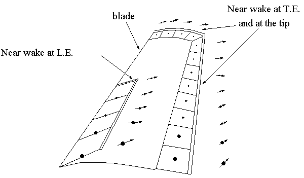
Figure 1: The separation model for a rotor blade.

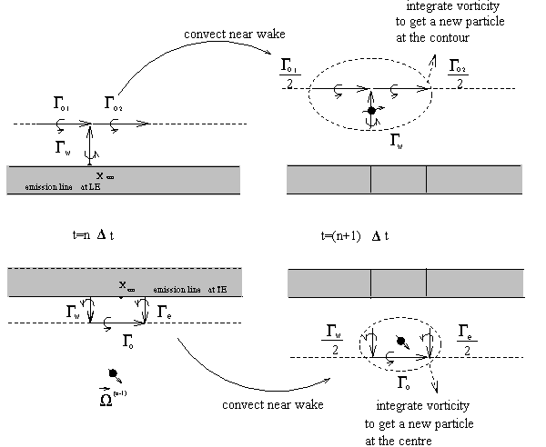
Figure 2: The formation of vortex particles.

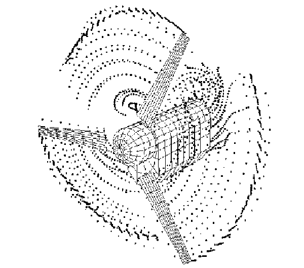
Figure 3:The computational configuration

3. THE LEADING EDGE SEPARATION MODEL

The stall condition is needed to determine the rate with which vorticity is shed along the leading edge of the blade or equivalently to determine the dipole intensitiesì_s of the leading edge near wakes. From a physical point of view this is a clearly viscous information which in our case is obtained by an empirical model. After testing many alternatives, finally a version of the ONERA model was kept. The model provides the change of circulation around an airfoil due to stallÃ_s as solution of a second order differential equation [4] :

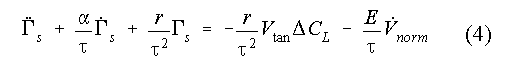
where,ô=2V_tan/c, c is the chord of the airfoil section, V_tan is the flow velocity parallel to the airfoil chord, V_norm is the flow velocity normal to the airfoil chord, ÄC_L is the difference between the steady potential lift coefficient and the steady state lift coefficient;á,r,E are empiric parameters.

In order to determine the angle of attackÄC_L at every strip of the blade is required. As reference angle the "attached" angle determined by a fully attached run is used. It is defined by the direction normal to the total (potential) force.

Equation (4) is applied to every strip along the span of the blade, closing the system of the equations. The dipole intensityì_s of the near wake elements at the leading edge is then given by the relation:

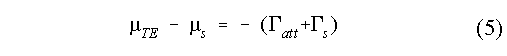
whereì_TE is the dipole intensity at the trailing edge of the strip and Ã_att is the attached circulation around the specific strip obtained by the fully attached run (See [7] for details).

4. RESULTS AND DISCUSSION

The proposed model was evaluated against measurements, carried out at Cranfield, on a small (D=3m , 340 RPM), three bladed stall regulated wind turbine [8]. Fig. 3 shows the computational configuration which also includes the nacelle of the wind turbine. In the same figure the first steps of the evolution of the wake are also presented. The nacelle is modelled as a bluff body with wake originating from its downstream edge. The model was run for several cases all yawed at high wind speeds in order to ensure the presence of stall. Results from a representative case are given in Fig. 4,5 corresponding to the 35% and 75% radial positions respectively. In every set of diagrams predictions are shown as a function othe azimuth angle (Fig. 4,5(a,b)) and of the angle of attack Fig. (4,5(c)). In the figures GENUVP and GENUVP+Stall correspond to results from the attached and stalled runs respectively.

Comparison of the predictions with the measurements shows that the model reproduces in a satisfactory way the physics of stall especially at the 75% section where stall is not very deep. Discrepancies appear in the predictions of the normal and tangential force at the 35% section which are due to the difficulty of simulating 3D viscous effects at the inboard sections of the blade under very deep stall conditions. At this section the shape of the variation is correct but there are level differences between measurements and predictions. The localised peak appearing in the azimuthal position of 270^o must be due to the elastic response of the blade to the excitation caused by the nacelle which shades the 35% section of the blade (Fig. 3) when it passes from this position. Worth noting are the changes in the position and the width of the loops as a result of the implementation of the stall model (Fig. 4,5(c)). At the inboard section the loop switches its sense from anticlockwise to clockwise (Fig. 4(c)). This is a typical viscous effect. The eight like shape of the loop at this section is due to the nacelle effect.

Measurements and predictions show that the presence of stall gives rise to significant ranges of variation of the normal force at the outboard section (Fig. 5(a)) which may affect the reliability of a wind turbine. As regards the tangential force the presence of stall changes significantly the shape and the mean value of the variation leaving the ranges practically unchanged. In order to better understand the impact of yaw induced stall on the fatigue loads of a rotor blade, an investigation of the influence of the different operational parameters including yaw misalignment was carried out for three wind turbines of different sizes: D=21m, D=30m, and D=37m. Indicative results are given in table (I) for a mean wind inflow of 14m/s. The equivalent blade loads for two different values of the turbulent intensity (T.I.=15% and T.I.=25%) and a yawed case ( 30 deg ) with T.I.=15% are presented whereas Fig. 6 shows the cumulative rainflow counting plot of the flapwise bending moment for the smallest blade.

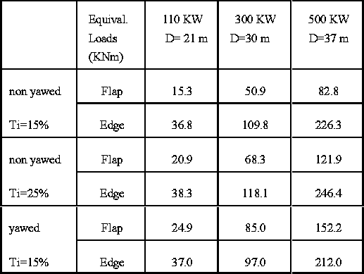
Table I: Equivalent loads for three different size blades.

It is clear that yaw misalignment charges significantly the loading of the blades, even more than a high value of the T.I. This is an important remark which should be specifically accounted for in the design and certification of a blade. It would be interesting to consider new airfoil shapes with stall

appearing at higher incidence [9].

In the present paper a new three dimensional advanced stall

model is proposed based on the double wake concept. It gives consistent predictions of the aerodynamic loads for rotors operating in yaw and its relatively low computational cost makes it attractive even for engineering applications.

The results from the parametric investigation indicate that yaw induced stall has a role comparative to that of extremely high turbulence intensity (25%).

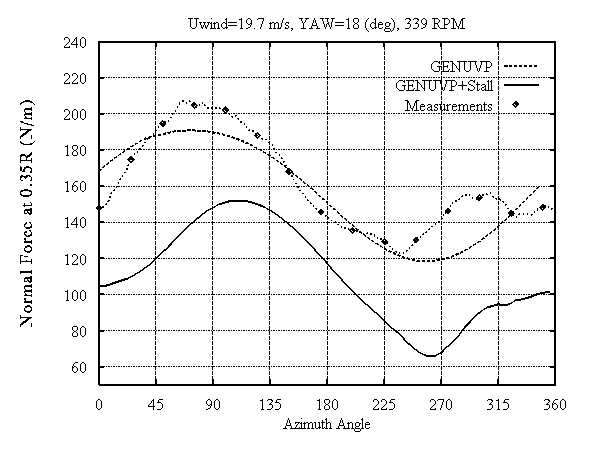
Figure 4a: Sectional Normal Force at 0.35R as function of the azimuthal position.

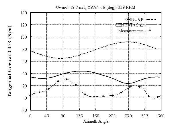Figure 4b: Sectional Tangential Force at 0.35R as function of the azimuthal position.

Figure 4c: Sectional Normal Force at 0.35R as function of the angle of attack. Dot indicates the starting point of the loop.

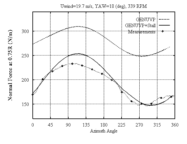
Figure 5a: Sectional Normal Force at 0.75R function of the azimuthal position.

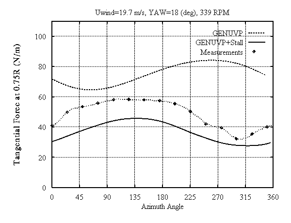
Figure 5b: Sectional Tangential Force at 0.75R as function of the azimuthal position.

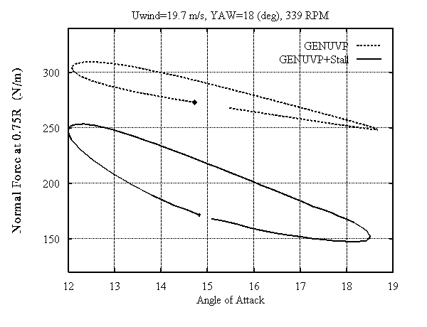
Figure 5c: Sectional Normal Force at 0.75R as function of the angle of attack. Dot indicates the starting point of the loop.

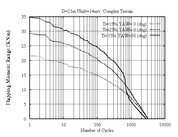
Figure 6: Rainflow counting plots.

ACKNOWLEDGEMENT

The present work was partially financed by the DG-XII of the CEU under the JOU2-CT93-0345 project.

REFERENCES

[1] Snel,H. and Schepers,J.G., Report ECN-C--94-107, (1994)

[2] Hansen,A.C. and Butterfield,C.P., Ann. Rev. Fluid Mechanics, (1993), Vol. 25, pp. 115-149

[3] Petot,D., Rech. Aerosp., (1989), paper no.5

[4] Leishman,J.G. and Beddoes,T.S., Proc. 42th Annual Forum of the American Helicopter society, (1986), Washington D.C., pp. 243-265

[5] AGARD-CP-552, "Aerodynamics and Aeroacoustics of Rotorcraft," Berlin (1995)

[6] Voutsinas,S.G., "Development of a New Generation of Design Tools for HAWT", Final Report of the JOU2-CT92-0113 CEU project, (1995)

[7] Voutsinas,S.G. and Riziotis,V.A., ASME Symposium on Vortex Methods and Vortex Flows, San Diego, (1996)

[8] Belia,J.M. and Hales,R.L., "An Experimental Investigation of HAWT Aerodynamics in Natural Conditions," Cranfield Institute of Technology, Final Report of the EN3W/0033/GB CEC project, (1990)

[9] Chaviaropoulos,P., Vossinis,A., Voutsinas, S., EUWEC'96, (1996)